Showing posts with label wireless communication. Show all posts

Thursday 8 August 2019

Outout backoff(OPBO) vs Input Backoff(IPBO) in RF Amplifier

Both the Output backoff(OPBO) and Input Backoff(IPBO) are used to determine the operating power levels required in a satellite transponder TWTA or RF Power Amplifier to function in linear region.

Output Back-Off (OPBO) is the power level at the output of RF amplifier relative to maximum output level possible using the RF amplifier.

EXAMPLE:
Maximum output level = +40dBm
Measured output level of RF Amplifier = +34dBm
Output Backoff(OPBO)= 6dB
Input Back-Off (IPBO) is the power level at the input of RF amplifier relative to input power which produces maximum output power.

Example:
Input power level causes max. output power = -20dBm
Actual input power level = -25dBm
Input backoff(IPBO)= 5dB
OPBO is used even to calculate inter-modulation distortion power levels at the output of TWTA/SSPA. For SSPA output backoff is same as 1dB compression point and for TWTA output backoff is same as saturated output power.

In a satellite link calculation, input backoff is calculated by taking difference between actual flux density and the saturated flux density. Also calculated Output backoff help calculated actual EIRP of the satellite.


Friday 2 August 2019

Set different energy levels to wireless nodes

You can set different initial energy to each wireless node separately. Your TCL script example is below.

set opt(initialenergy) 1000 ; # Initial energy in Joules

# Define Mobile Node Configurations
$ns node-config -adhocRouting $val(rp) \
-llType $val(ll) \
-macType $val(mac) \
-ifqType $val(ifq) \
-ifqLen $val(ifqlen) \
-antType $val(ant) \
-propType $val(prop) \
-phyType $val(netif) \
-channelType $val(chan) \
-topoInstance $topo \
-agentTrace ON \
-routerTrace ON \
-macTrace ON \
-movementTrace ON \
-energyModel $opt(energymodel) \
-idlePower 1.0 \
-rxPower 1.0 \
-txPower 1.0 \
-sleepPower 0.001 \
-transitionPower 0.2 \
-transitionTime 0.005 \
-initialEnergy $opt(initialenergy)

....
....
set node_(0) [$ns node] # This will be generate node with initial energy 1000 Joules

$ns node-config -initialEnergy 500
set node_(1) [$ns node]


$ns node-config -initialEnergy 20
set node_(2) [$ns node]

$ns node-config -initialEnergy 30
set node_(3) [$ns node]

$ns node-config -initialEnergy 100
set node_(4) [$ns node]

...


You can find an example of 5 Nodes with different energy levels / AODV Routing Protocol in NS 2.35 below.
# wireless-qeaodv.tcl
# 5 Nodes with different energy levels / AODV Routing Protocol Example

# ======================================================================
# Define Values
# ======================================================================
set val(chan) Channel/WirelessChannel ;
set val(prop) Propagation/TwoRayGround ;
set val(ant) Antenna/OmniAntenna ;
set val(ll) LL ;
set val(ifq) Queue/DropTail/PriQueue ;
set val(ifqlen) 50 ;
set val(netif) Phy/WirelessPhy ;
set val(mac) Mac/802_11 ;
set val(rp) AODV ;
set val(nn) 5 ;
set opt(energymodel) EnergyModel ;
set opt(initialenergy) 1000 ; # Initial energy in Joules
set opt(lm) "off" ;# log movement
set opt(logenergy) "on" ;# log energy every 150 seconds

set val(x) 500 ;
set val(y) 500 ;
set val(stop) 60;
set filename $val(rp)_$val(nn)_$val(x)_$val(y);
set ns [new Simulator]

# open trace file
set tracefd [open $filename.tr w]
$ns trace-all $tracefd

#Open the nam trace file
set namtrace [open $filename.nam w]
$ns namtrace-all-wireless $namtrace $val(x) $val(y)


set WirelessNewTrace_ ON
#set AgentTrace ON
#set RouterTrace OFF
#set MacTrace ON

# ------------------------------------------------------------------------------
# Ağ topolojisi tanımı
# ------------------------------------------------------------------------------
set topo [new Topography]
$topo load_flatgrid $val(x) $val(y)

# General Operations Director (GOD)
create-god $val(nn)

# nn miktarınca düğüm [$val(nn)] oluştur ve kanala ilişkilendir.
set chan_1 [new $val(chan)]


# düğümleri konfigure et
$ns node-config -adhocRouting $val(rp) \
-llType $val(ll) \
-macType $val(mac) \
-ifqType $val(ifq) \
-ifqLen $val(ifqlen) \
-antType $val(ant) \
-propType $val(prop) \
-phyType $val(netif) \
-channelType $val(chan) \
-topoInstance $topo \
-agentTrace ON \
-routerTrace ON \
-macTrace ON \
-movementTrace ON \
-energyModel $opt(energymodel) \
-idlePower 1.0 \
-rxPower 1.0 \
-txPower 1.0 \
-sleepPower 0.001 \
-transitionPower 0.2 \
-transitionTime 0.005 \
-initialEnergy $opt(initialenergy)

#for {set i 0} {$i < $val(nn) } { incr i } {
# set node_($i) [$ns node]
# $node_($i) random-motion 0 ;# disable random motion
#}

# Set initialEnergy values for Nodes
$ns node-config -initialEnergy 500
set node_(0) [$ns node]
$node_(0) color blue
$node_(0) shape box
$node_(0) label "Source"

# Set initial_node_pos
$node_(0) set X_ 40.0
$node_(0) set Y_ 280.0


$ns node-config -initialEnergy 500
set node_(1) [$ns node]

$ns node-config -initialEnergy 20
set node_(2) [$ns node]

$ns node-config -initialEnergy 20
set node_(3) [$ns node]

$ns node-config -initialEnergy 100
set node_(4) [$ns node]


# $node color [color] ;# sets color of node
# $node shape [shape] ;# sets shape of node
# $node label [label] ;# sets label on node
# $node label-color [lcolor] ;# sets color of label
# $node label-at [ldirection] ;# sets position of label
# $node add-mark [name] [color] [shape] ;# adds a mark to node
# $node delete-mark [name] ;# deletes mark from node

$node_(1) set X_ 420.0
$node_(1) set Y_ 280.0
$node_(1) color "red"
$node_(1) label "Destination"

$node_(2) set X_ 220.0
$node_(2) set Y_ 380.0
$node_(2) color "green"

$node_(3) set X_ 360.0
$node_(3) set Y_ 280.0
$node_(3) color "green"

$node_(4) set X_ 220.0
$node_(4) set Y_ 180.0
$node_(4) color "green"


for {set i 0} {$i < $val(nn) } { incr i } {
$ns initial_node_pos $node_($i) 30;
}


set udp [new Agent/UDP]
$ns attach-agent $node_(0) $udp
set null [new Agent/Null]
$ns attach-agent $node_(1) $null
$ns connect $udp $null
$udp set fid_ 1

set cbr [new Application/Traffic/CBR]
$cbr attach-agent $udp
$cbr set type_ CBR
$cbr set packetSize_ 48; # 48 byte 384bit
$cbr set rate_ 64000; # 0.064Mb || 64kb || 64000bit || bits per second
# interval_=0.0060000000000000001 || bit per second || 384/64000
# Packets in one second = 64000/384= 166,6packet

$cbr set random_ false


$ns at 10.0 "$cbr start"


for {set i 0} {$i < $val(nn) } { incr i } {
$ns at $val(stop) "$node_($i) reset";
}

$ns at 60.0 "$cbr stop"
# ------------------------------------------------------------------------------
# nam ve simulation end
# ------------------------------------------------------------------------------
# $ns at 15 "$node_(0) print_rtable"
$ns at $val(stop) "$ns nam-end-wireless $val(stop)"
#$ns at $val(stop) "$awk -f _packet.awk AODV_5_500_500.tr"
$ns at 70 "stop"
$ns at 70 "puts "end simulation" ; $ns halt"


proc stop {} {
global ns tracefd namtrace filename
$ns flush-trace
close $tracefd
close $namtrace
exec nam $filename.nam; #Execute nam on the trace file
exec awk -f _packet.awk $filename.tr
}

$ns run

Tuesday 16 July 2019

Difference between Spin stabilization and three-axis stabilization

Spin stabilization and three-axis stabilization are two methods that are used to orient satellites. With spin stabilization, the entire spacecraft rotates around its own vertical axis, spinning like a top. This keeps the spacecraft's orientation in space under control. The advantage of spin stabilization is that it is a very simple way to keep the spacecraft pointed in a certain direction. The spinning spacecraft resists perturbing forces, which tend to be small in space, just like a gyroscope or a top. Designers of early satellites used spin-stabilization for their satellites, which most often have a cylinder shape and rotate at one revolution every second. A disadvantage to this type of stabilization is that the satellite cannot use large solar arrays to obtain power from the Sun. Thus, it requires large amounts of battery power. Another disadvantage of spin stabilization is that the instruments or antennas also must perform “despin” maneuvers so that antennas or optical instruments point at their desired targets. Spin stabilization was used for NASA's Pioneer 10 and 11 spacecraft, the Lunar Prospector, and the Galileo Jupiter orbiter.

With three-axis stabilization, satellites have small spinning wheels, called reaction wheels or momentum wheels, that rotate so as to keep the satellite in the desired orientation in relation to the Earth and the Sun. If satellite sensors detect that the satellite is moving away from the proper orientation, the spinning wheels speed up or slow down to return the satellite to its correct position. Some spacecraft may also use small propulsion-system thrusters to continually nudge the spacecraft back and forth to keep it within a range of allowed positions. Voyagers 1 and 2 stay in position using 3-axis stabilization. An advantage of 3-axis stabilization is that optical instruments and antennas can point at desired targets without having to perform “despin” maneuvers.

Monday 8 July 2019

Spread spectrum

A collective class of signaling techniques are employed before transmitting a signal to provide a secure communication, known as the Spread Spectrum Modulation. The main advantage of spread spectrum communication technique is to prevent “interference” whether it is intentional or unintentional.
The signals modulated with these techniques are hard to interfere and cannot be jammed. An intruder with no official access is never allowed to crack them. Hence, these techniques are used for military purposes. These spread spectrum signals transmit at low power density and has a wide spread of signals.

Pseudo-Noise Sequence

A coded sequence of 1s and 0s with certain auto-correlation properties, called as Pseudo-Noise coding sequence is used in spread spectrum techniques. It is a maximum-length sequence, which is a type of cyclic code.

Narrow-band and Spread-spectrum Signals

Both the Narrow band and Spread spectrum signals can be understood easily by observing their frequency spectrum as shown in the following figures.

Narrow-band Signals

The Narrow-band signals have the signal strength concentrated as shown in the following frequency spectrum figure.
Narrow-band Signals
Following are some of its features −
  • Band of signals occupy a narrow range of frequencies.
  • Power density is high.
  • Spread of energy is low and concentrated.
Though the features are good, these signals are prone to interference.

Spread Spectrum Signals

The spread spectrum signals have the signal strength distributed as shown in the following frequency spectrum figure.
Spread Spectrum Signals
Following are some of its features −
  • Band of signals occupy a wide range of frequencies.
  • Power density is very low.
  • Energy is wide spread.
With these features, the spread spectrum signals are highly resistant to interference or jamming. Since multiple users can share the same spread spectrum bandwidth without interfering with one another, these can be called as multiple access techniques.

FHSS and DSSS / CDMA

Spread spectrum multiple access techniques uses signals which have a transmission bandwidth of a magnitude greater than the minimum required RF bandwidth.
These are of two types.
  • Frequency Hopped Spread Spectrum (FHSS)
  • Direct Sequence Spread Spectrum (DSSS)

Frequency Hopped Spread Spectrum (FHSS)

This is frequency hopping technique, where the users are made to change the frequencies of usage, from one to another in a specified time interval, hence called as frequency hopping. For example, a frequency was allotted to sender 1 for a particular period of time. Now, after a while, sender 1 hops to the other frequency and sender 2 uses the first frequency, which was previously used by sender 1. This is called as frequency reuse.
The frequencies of the data are hopped from one to another in order to provide a secure transmission. The amount of time spent on each frequency hop is called as Dwell time.

Direct Sequence Spread Spectrum (DSSS)

Whenever a user wants to send data using this DSSS technique, each and every bit of the user data is multiplied by a secret code, called as chipping code. This chipping code is nothing but the spreading code which is multiplied with the original message and transmitted. The receiver uses the same code to retrieve the original message.

Comparison between FHSS and DSSS/CDMA

Both the spread spectrum techniques are popular for their characteristics. To have a clear understanding, let us take a look at their comparisons.
FHSSDSSS / CDMA
Multiple frequencies are usedSingle frequency is used
Hard to find the user’s frequency at any instant of timeUser frequency, once allotted is always the same
Frequency reuse is allowedFrequency reuse is not allowed
Sender need not waitSender has to wait if the spectrum is busy
Power strength of the signal is highPower strength of the signal is low
Stronger and penetrates through the obstaclesIt is weaker compared to FHSS
It is never affected by interferenceIt can be affected by interference
It is cheaperIt is expensive
This is the commonly used techniqueThis technique is not frequently used

Advantages of Spread Spectrum

Following are the advantages of spread spectrum −
  • Cross-talk elimination
  • Better output with data integrity
  • Reduced effect of multipath fading
  • Better security
  • Reduction in noise
  • Co-existence with other systems
  • Longer operative distances
  • Hard to detect
  • Not easy to demodulate/decode
  • Difficult to jam the signals
Although spread spectrum techniques were originally designed for military uses, they are now being used widely for commercial purpose.

Monday 1 July 2019

Data communication Networking-Physical layer

Switching is process to forward packets coming in from one port to a port leading towards the destination. When data comes on a port it is called ingress, and when data leaves a port or goes out it is called egress. A communication system may include number of switches and nodes. At broad level, switching can be divided into two major categories:
  • Connectionless: The data is forwarded on behalf of forwarding tables. No previous handshaking is required and acknowledgements are optional.
  • Connection Oriented:  Before switching data to be forwarded to destination, there is a need to pre-establish circuit along the path between both endpoints. Data is then forwarded on that circuit. After the transfer is completed, circuits can be kept for future use or can be turned down immediately.

Circuit Switching

When two nodes communicate with each other over a dedicated communication path, it is called circuit switching.There 'is a need of pre-specified route from which data will travels and no other data is permitted.In circuit switching, to transfer the data, circuit must be established so that the data transfer can take place.
Circuits can be permanent or temporary. Applications which use circuit switching may have to go through three phases:
  • Establish a circuit
  • Transfer the data
  • Disconnect the circuit
Circuit Switching
Circuit switching was designed for voice applications. Telephone is the best suitable example of circuit switching. Before a user can make a call, a virtual path between caller and callee is established over the network.

Message Switching

This technique was somewhere in middle of circuit switching and packet switching. In message switching, the whole message is treated as a data unit and is switching / transferred in its entirety.
A switch working on message switching, first receives the whole message and buffers it until there are resources available to transfer it to the next hop. If the next hop is not having enough resource to accommodate large size message, the message is stored and switch waits.
Message Switching
This technique was considered substitute to circuit switching. As in circuit switching the whole path is blocked for two entities only. Message switching is replaced by packet switching. Message switching has the following drawbacks:
  • Every switch in transit path needs enough storage to accommodate entire message.
  • Because of store-and-forward technique and waits included until resources are available, message switching is very slow.
  • Message switching was not a solution for streaming media and real-time applications.

Packet Switching

Shortcomings of message switching gave birth to an idea of packet switching. The entire message is broken down into smaller chunks called packets. The switching information is added in the header of each packet and transmitted independently.
It is easier for intermediate networking devices to store small size packets and they do not take much resources either on carrier path or in the internal memory of switches.
Packet Switching
Packet switching enhances line efficiency as packets from multiple applications can be multiplexed over the carrier. The internet uses packet switching technique. Packet switching enables the user to differentiate data streams based on priorities. Packets are stored and forwarded according to their priority to provide quality of service.

Multiplexing -Physical layer

Multiplexing is a technique by which different analog and digital streams of transmission can be simultaneously processed over a shared link. Multiplexing divides the high capacity medium into low capacity logical medium which is then shared by different streams.
Communication is possible over the air (radio frequency), using a physical media (cable), and light (optical fiber). All mediums are capable of multiplexing.
When multiple senders try to send over a single medium, a device called Multiplexer divides the physical channel and allocates one to each. On the other end of communication, a De-multiplexer receives data from a single medium, identifies each, and sends to different receivers.

Frequency Division Multiplexing

When the carrier is frequency, FDM is used. FDM is an analog technology. FDM divides the spectrum or carrier bandwidth in logical channels and allocates one user to each channel. Each user can use the channel frequency independently and has exclusive access of it. All channels are divided in such a way that they do not overlap with each other. Channels are separated by guard bands. Guard band is a frequency which is not used by either channel.
Frequency Division Multiplexing

Time Division Multiplexing

TDM is applied primarily on digital signals but can be applied on analog signals as well. In TDM the shared channel is divided among its user by means of time slot. Each user can transmit data within the provided time slot only. Digital signals are divided in frames, equivalent to time slot i.e. frame of an optimal size which can be transmitted in given time slot.
TDM works in synchronized mode. Both ends, i.e. Multiplexer and De-multiplexer are timely synchronized and both switch to next channel simultaneously.
Time Division Multiplexing
When channel A transmits its frame at one end,the De-multiplexer provides media to channel A on the other end.As soon as the channel A’s time slot expires, this side switches to channel B. On the other end, the De-multiplexer works in a synchronized manner and provides media to channel B. Signals from different channels travel the path in interleaved manner.

Wavelength Division Multiplexing

Light has different wavelength (colors). In fiber optic mode, multiple optical carrier signals are multiplexed into an optical fiber by using different wavelengths. This is an analog multiplexing technique and is done conceptually in the same manner as FDM but uses light as signals.
Wavelength Division Multiplexing
Further, on each wavelength time division multiplexing can be incorporated to accommodate more data signals.

Code Division Multiplexing

Multiple data signals can be transmitted over a single frequency by using Code Division Multiplexing. FDM divides the frequency in smaller channels but CDM allows its users to full bandwidth and transmit signals all the time using a unique code. CDM uses orthogonal codes to spread signals.
Each station is assigned with a unique code, called chip. Signals travel with these codes independently, inside the whole bandwidth.The receiver knows in advance the chip code signal it has to receive.

Transmission media-Physical Layer

The transmission media is nothing but the physical media over which communication takes place in computer networks.

Magnetic Media

One of the most convenient way to transfer data from one computer to another, even before the birth of networking, was to save it on some storage media and transfer physical from one station to another. Though it may seem old-fashion way in today’s world of high speed internet, but when the size of data is huge, the magnetic media comes into play.
For example, a bank has to handle and transfer huge data of its customer, which stores a backup of it at some geographically far-away place for security reasons and to keep it from uncertain calamities. If the bank needs to store its huge backup data then its,transfer through internet is not feasible.The WAN links may not support such high speed.Even if they do; the cost too high to afford.
In these cases, data backup is stored onto magnetic tapes or magnetic discs, and then shifted physically at remote places.

Twisted Pair Cable

A twisted pair cable is made of two plastic insulated copper wires twisted together to form a single media. Out of these two wires, only one carries actual signal and another is used for ground reference. The twists between wires are helpful in reducing noise (electro-magnetic interference) and crosstalk.

There are two types of twisted pair cables:
  • Shielded Twisted Pair (STP) Cable
  • Unshielded Twisted Pair (UTP) Cable
STP cables comes with twisted wire pair covered in metal foil. This makes it more indifferent to noise and crosstalk.
UTP has seven categories, each suitable for specific use. In computer networks, Cat-5, Cat-5e, and Cat-6 cables are mostly used. UTP cables are connected by RJ45 connectors.

Coaxial Cable

Coaxial cable has two wires of copper. The core wire lies in the center and it is made of solid conductor.The core is enclosed in an insulating sheath.The second wire is wrapped around over the sheath and that too in turn encased by insulator sheath.This all is covered by plastic cover.
Coaxial Cable
Because of its structure,the coax cable is capable of carrying high frequency signals than that of twisted pair cable.The wrapped structure provides it a good shield against noise and cross talk. Coaxial cables provide high bandwidth rates of up to 450 mbps.
There are three categories of coax cables namely, RG-59 (Cable TV), RG-58 (Thin Ethernet), and RG-11 (Thick Ethernet). RG stands for Radio Government.
Cables are connected using BNC connector and BNC-T. BNC terminator is used to terminate the wire at the far ends.

Power Lines

Power Line communication (PLC) is Layer-1 (Physical Layer) technology which uses power cables to transmit data signals.In PLC, modulated data is sent over the cables. The receiver on the other end de-modulates and interprets the data.
Because power lines are widely deployed, PLC can make all powered devices controlled and monitored. PLC works in half-duplex.
There are two types of PLC:
  • Narrow band PLC
  • Broad band PLC
Narrow band PLC provides lower data rates up to 100s of kbps, as they work at lower frequencies (3-5000 kHz).They can be spread over several kilometers.
Broadband PLC provides higher data rates up to 100s of Mbps and works at higher frequencies (1.8 – 250 MHz).They cannot be as much extended as Narrowband PLC.

Fiber Optics

Fiber Optic works on the properties of light. When light ray hits at critical angle it tends to refracts at 90 degree. This property has been used in fiber optic. The core of fiber optic cable is made of high quality glass or plastic. From one end of it light is emitted, it travels through it and at the other end light detector detects light stream and converts it to electric data.
Fiber Optic provides the highest mode of speed. It comes in two modes, one is single mode fiber and second is multimode fiber. Single mode fiber can carry a single ray of light whereas multimode is capable of carrying multiple beams of light.
Fiber Optics
Fiber Optic also comes in unidirectional and bidirectional capabilities. To connect and access fiber optic special type of connectors are used. These can be Subscriber Channel (SC), Straight Tip (ST), or MT-RJ.

Analog Transmission-Physical Layer

To send the digital data over an analog media, it needs to be converted into analog signal.There can be two cases according to data formatting.
Bandpass:The filters are used to filter and pass frequencies of interest. A bandpass is a band of frequencies which can pass the filter.
Low-pass: Low-pass is a filter that passes low frequencies signals.
When digital data is converted into a bandpass analog signal, it is called digital-to-analog conversion. When low-pass analog signal is converted into bandpass analog signal, it is called analog-to-analog conversion.

Digital-to-Analog Conversion

When data from one computer is sent to another via some analog carrier, it is first converted into analog signals. Analog signals are modified to reflect digital data.
An analog signal is characterized by its amplitude, frequency, and phase. There are three kinds of digital-to-analog conversions:
  • Amplitude Shift Keying
    In this conversion technique, the amplitude of analog carrier signal is modified to reflect binary data.
    Amplitude Shift Keying
    When binary data represents digit 1, the amplitude is held; otherwise it is set to 0. Both frequency and phase remain same as in the original carrier signal.
  • Frequency Shift Keying
    In this conversion technique, the frequency of the analog carrier signal is modified to reflect binary data.
    Frequency Shift Keying
    This technique uses two frequencies, f1 and f2. One of them, for example f1, is chosen to represent binary digit 1 and the other one is used to represent binary digit 0. Both amplitude and phase of the carrier wave are kept intact.
  • Phase Shift Keying
    In this conversion scheme, the phase of the original carrier signal is altered to reflect the binary data.
    Phase Shift Keying
    When a new binary symbol is encountered, the phase of the signal is altered. Amplitude and frequency of the original carrier signal is kept intact.
  • Quadrature Phase Shift Keying
    QPSK alters the phase to reflect two binary digits at once. This is done in two different phases. The main stream of binary data is divided equally into two sub-streams. The serial data is converted in to parallel in both sub-streams and then each stream is converted to digital signal using NRZ technique. Later, both the digital signals are merged together.

Analog-to-Analog Conversion

Analog signals are modified to represent analog data. This conversion is also known as Analog Modulation. Analog modulation is required when bandpass is used. Analog to analog conversion can be done in three ways:
Analog Modulation
  • Amplitude Modulation
    In this modulation, the amplitude of the carrier signal is modified to reflect the analog data.
    Amplitude Modulation
    Amplitude modulation is implemented by means of a multiplier. The amplitude of modulating signal (analog data) is multiplied by the amplitude of carrier frequency, which then reflects analog data.
    The frequency and phase of carrier signal remain unchanged.
  • Frequency Modulation
    In this modulation technique, the frequency of the carrier signal is modified to reflect the change in the voltage levels of the modulating signal (analog data).
    Frequency Modulation
    The amplitude and phase of the carrier signal are not altered.
  • Phase Modulation
    In the modulation technique, the phase of carrier signal is modulated in order to reflect the change in voltage (amplitude) of analog data signal.
    Phase Modulation
    Phase modulation is practically similar to Frequency Modulation, but in Phase modulation frequency of the carrier signal is not increased. Frequency of carrier is signal is changed (made dense and sparse) to reflect voltage change in the amplitude of modulating signal.

Digital Transmission

Data or information can be stored in two ways, analog and digital. For a computer to use the data, it must be in discrete digital form.Similar to data, signals can also be in analog and digital form. To transmit data digitally, it needs to be first converted to digital form.

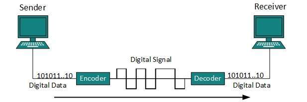
Digital-to-Digital Conversion

This section explains how to convert digital data into digital signals. It can be done in two ways, line coding and block coding. For all communications, line coding is necessary whereas block coding is optional.

Line Coding

The process for converting digital data into digital signal is said to be Line Coding. Digital data is found in binary format.It is represented (stored) internally as series of 1s and 0s.
Line Coding
Digital signal is denoted by discreet signal, which represents digital data.There are three types of line coding schemes available:
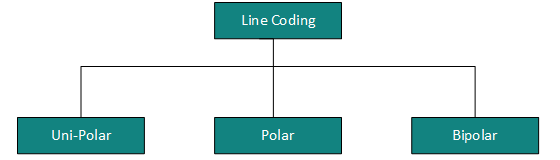
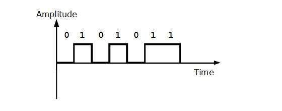
Line Coding

Uni-polar Encoding

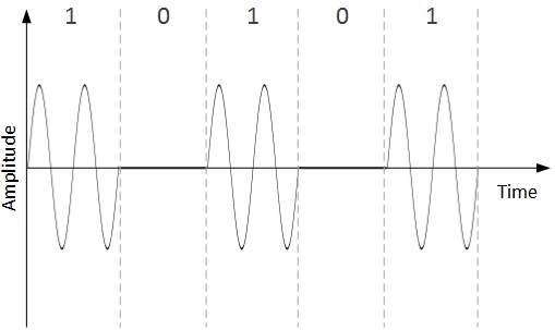
Unipolar encoding schemes use single voltage level to represent data. In this case, to represent binary 1, high voltage is transmitted and to represent 0, no voltage is transmitted. It is also called Unipolar-Non-return-to-zero, because there is no rest condition i.e. it either represents 1 or 0.
UniPolar NRZ Encoding

Polar Encoding

Polar encoding scheme uses multiple voltage levels to represent binary values. Polar encodings is available in four types:
  • Polar Non-Return to Zero (Polar NRZ)
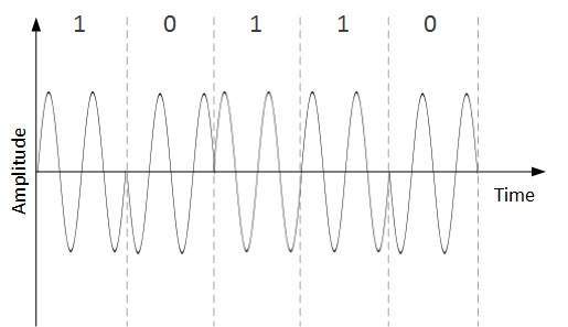
    It uses two different voltage levels to represent binary values. Generally, positive voltage represents 1 and negative value represents 0. It is also NRZ because there is no rest condition.
    NRZ scheme has two variants: NRZ-L and NRZ-I.
    Unipolar NRZ
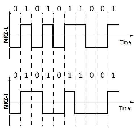
    NRZ-L changes voltage level at when a different bit is encountered whereas NRZ-I changes voltage when a 1 is encountered.
  • Return to Zero (RZ)

    Problem with NRZ is that the receiver cannot conclude when a bit ended and when the next bit is started, in case when sender and receiver’s clock are not synchronized.
    Return-to-Zero
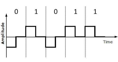
    RZ uses three voltage levels, positive voltage to represent 1, negative voltage to represent 0 and zero voltage for none. Signals change during bits not between bits.
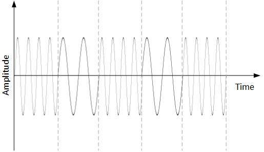
  • Manchester

    This encoding scheme is a combination of RZ and NRZ-L. Bit time is divided into two halves. It transits in the middle of the bit and changes phase when a different bit is encountered.
  • Differential Manchester

    This encoding scheme is a combination of RZ and NRZ-I. It also transit at the middle of the bit but changes phase only when 1 is encountered.
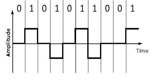
Bipolar Encoding

Bipolar encoding uses three voltage levels, positive, negative and zero. Zero voltage represents binary 0 and bit 1 is represented by altering positive and negative voltages.

Block Coding

To ensure accuracy of the received data frame redundant bits are used. For example, in even-parity, one parity bit is added to make the count of 1s in the frame even. This way the original number of bits is increased. It is called Block Coding.
Block coding is represented by slash notation, mB/nB.Means, m-bit block is substituted with n-bit block where n > m. Block coding involves three steps:
  • Division,
  • Substitution
  • Combination.
After block coding is done, it is line coded for transmission.

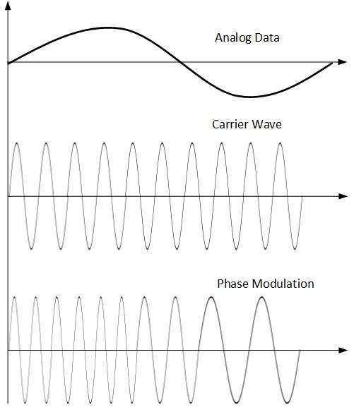
Analog-to-Digital Conversion

Microphones create analog voice and camera creates analog videos, which are treated is analog data. To transmit this analog data over digital signals, we need analog to digital conversion.
Analog data is a continuous stream of data in the wave form whereas digital data is discrete. To convert analog wave into digital data, we use Pulse Code Modulation (PCM).
PCM is one of the most commonly used method to convert analog data into digital form. It involves three steps:
  • Sampling
  • Quantization
  • Encoding.

Sampling

Sampling
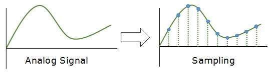
The analog signal is sampled every T interval. Most important factor in sampling is the rate at which analog signal is sampled. According to Nyquist Theorem, the sampling rate must be at least two times of the highest frequency of the signal.

Quantization

Quantization
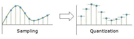
Sampling yields discrete form of continuous analog signal. Every discrete pattern shows the amplitude of the analog signal at that instance. The quantization is done between the maximum amplitude value and the minimum amplitude value. Quantization is approximation of the instantaneous analog value.

Encoding

Encoding
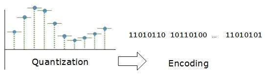
In encoding, each approximated value is then converted into binary format.

Transmission Modes

The transmission mode decides how data is transmitted between two computers.The binary data in the form of 1s and 0s can be sent in two different modes: Parallel and Serial.

Parallel Transmission

Parallel Transmission
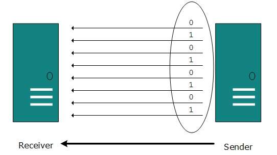
The binary bits are organized in-to groups of fixed length. Both sender and receiver are connected in parallel with the equal number of data lines. Both computers distinguish between high order and low order data lines. The sender sends all the bits at once on all lines.Because the data lines are equal to the number of bits in a group or data frame, a complete group of bits (data frame) is sent in one go. Advantage of Parallel transmission is high speed and disadvantage is the cost of wires, as it is equal to the number of bits sent in parallel.
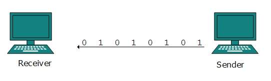
Serial Transmission

In serial transmission, bits are sent one after another in a queue manner. Serial transmission requires only one communication channel.
Serial Transmission
Serial transmission can be either asynchronous or synchronous.

Asynchronous Serial Transmission

It is named so because there’is no importance of timing. Data-bits have specific pattern and they help receiver recognize the start and end data bits.For example, a 0 is prefixed on every data byte and one or more 1s are added at the end.
Two continuous data-frames (bytes) may have a gap between them.

Synchronous Serial Transmission

Timing in synchronous transmission has importance as there is no mechanism followed to recognize start and end data bits.There is no pattern or prefix/suffix method. Data bits are sent in burst mode without maintaining gap between bytes (8-bits). Single burst of data bits may contain a number of bytes. Therefore, timing becomes very important.
It is up to the receiver to recognize and separate bits into bytes.The advantage of synchronous transmission is high speed, and it has no overhead of extra header and footer bits as in asynchronous transmission.