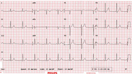
I recently had a medical checkup that included an ECG (electro-cardiograph).
This is what my ECG looked like:

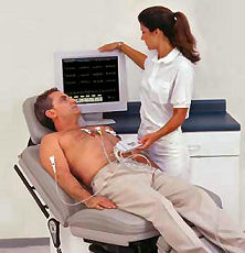
The electrodes are connected to various parts of your anatomy (chest, legs, arms, feet) and voltage differences over time are measured to give the ECG readout.
The horizontal axis of the ECG printout represents time and the vertical axis is the amplitude of the voltage.
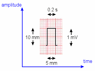
Amplitude units are millivolts (mV) and on the graph, 1 mV = 10 mm high.
The time scale is 25 mm = 1 second (or 1 mm per 0.04 seconds on the graph).
So here's my readout for Lead II, representing the voltage between the positive electrode on my left leg and the electrode on my right arm. Each thicker red vertical line represents a time of 1 second.

Apparently (according to the doctor), this indicates my heart is quite healthy.
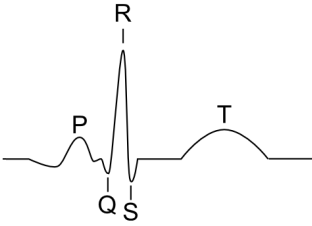
In more detail, the features of the repeated pulse we are looking at are as follows.
[Image source: T. Burke]
The P wave is caused by contraction of the right atrium followed by the left atrium (the chambers at the top of the heart).
The QRS complex represent the point in time when most of the heart muscles are in action, so has highest amplitude.
The T wave represents the polarization of the ventricles (the chambers at the bottom of the heart).

Human heart showing atria and ventricles.
[Image by UCSD, source page no longer available]
Modeling the Heartbeat Using Fourier Series
A heartbeat is roughly regular (if it isn't, it indicates something is wrong). Mathematically, we say something that repeats regularly is periodic.
Such waves can be represented using a Fourier Series.
Assumptions
In my case, my heart rate was about 70 beats per minute. For the sake of simplicity, I'll assume 60 beats per minute or 1 per second. So the period = 1 second = 1000 milliseconds.
Also for simplicity, I will only model the R wave for this article. To get a more accurate model for the heartbeat, I would just need to do a similar process for the P, Q, S and T waves and add them to my model.
I observed that my R wave was about 2.5 mV high and lasted for a total of 40 ms. The shape of the R wave is almost triangular and so I could have used straight lines for my model, but these don't give us a smooth curve (especially at the top - it must be continuously differentiable).
A better approach is to use a polynomial (where the ascending and descending lines are close enough to being straight), so my model is as follows (the time units are milliseconds):
f(t) = -0.0000156(t − 20)⁴ + 2.5
f(t) = f(t + 1000)
Explanation of the Model
The model is based on a quartic (power 4) since this will give me close to the shape I need (a parabola would be too broad). I'm using similar thinking to what I was doing in this article, where I move a curve around to where I want it.
The (t − 20) term comes from deciding the curve should start at (0,0), (which makes our lives easier), it will pass through (40,0) since the pulse is 40 ms long, and be centered on t = 20.
The "+2.5" comes from the fact the amplitude of the pulse is 2.5 mV.
The -0.0000156 comes from solving the following for a when t = 0.
a(t − 20)⁴ + 2.5 = 0.
The "f(t) = f(t + 1000)" part means the function (pulse in this case) is repeated every 1000 ms.
Graph of the Model
This is the graph of part of one period (the part above the t-axis from t = 0 to t = 40):

Of course. this is just one pulse. How do we produce a graph that repeats this pulse at regular intervals?
This is where we use Fourier Series.
I'll spare you all the details, but essentially the Fourier Series is an infinite series involving trigonometric terms. When all the terms are added, you get a mathematical model of the original periodic function.
To obtain the Fourier Series, wee need to find the mean value, a0, and 2 coefficient expressions involving n, an and bn which are multiplied by trigonometric terms and summed for n = 1 to infinity.
Mean Value Term
a0 is obtained by integration as follows (L is half of the period):
(The section of the curve we need for this part of the problem is from t = 0to t = 40, so that's why we chose those values for the limits of integration in the second last line.)
First Coefficient Term, an
Next, we compute an:
The answer for this integral is pretty ugly. I've included it in the PDF solution.
Second Coefficient Term, bn
Now for bn:
Once again, I have spared you from the full details.
Finally, we put it all together and obtain the Fourier Series for our simple model of a heart beat:


When we graph this for just the first 5 terms (n = 1 to 5), we can see the beginnings of a regular 1-second heart beat.

The above graph shows the "noise" you get in a Fourier Series expansion, especially if you haven't taken enough terms.
Taking more terms (this time, adding the first 100 terms) gives us the following, and we see we get a reasonable approximation for a regular R wave with period 1 second.

I added the T wave for this next model (in blue).
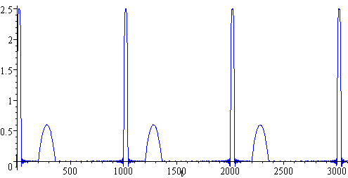
I used a parabola for the T wave because the shape of the T wave is broader than the shape of the R wave.
We could keep going, adding the P, Q and S waves to get an even better model.
What have we done?
We have taken a single spike representing one R wave of my heartbeat. We then found a formula that repeats our spike at regular time intervals. The Fourier Series (an infinite sum of trigonometric terms) gave us that formula.
Finally, we added the T wave, using the same theory as before.
Fourier Series is very useful in electronics and acoustics, where waveforms are periodic.
